This article discusses using Solver, a Microsoft Excel add-in program you can use for what-if analysis, to determine an optimal product mix.
Companies often need to determine the quantity of each product to produce on a monthly basis. In its simplest form, the product mix problem involves how to determine the amount of each product that should be produced during a month to maximize profits. Product mix must usually adhere to the following constraints:
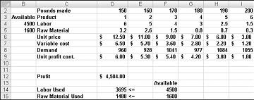
Let’s now solve the following example of the product mix problem. You can find the solution to this problem in the file Prodmix.xlsx, shown in Figure 27-1.

Let’s say we work for a drug company that produces six different products at their plant. Production of each product requires labor and raw material. Row 4 in Figure 27-1 shows the hours of labor needed to produce a pound of each product, and row 5 shows the pounds of raw material needed to produce a pound of each product. For example, producing a pound of Product 1 requires six hours of labor and 3.2 pounds of raw material. For each drug, the price per pound is given in row 6, the unit cost per pound is given in row 7, and the profit contribution per pound is given in row 9. For example, Product 2 sells for $11.00 per pound, incurs a unit cost of $5.70 per pound, and contributes $5.30 profit per pound. The month’s demand for each drug is given in row 8. For example, demand for Product 3 is 1041 pounds. This month, 4500 hours of labor and 1600 pounds of raw material are available. How can this company maximize its monthly profit?
If we knew nothing about Excel Solver, we would attack this problem by constructing a worksheet to track profit and resource usage associated with the product mix. Then we would use trial and error to vary the product mix to optimize profit without using more labor or raw material than is available, and without producing any drug in excess of demand. We use Solver in this process only at the trial-and-error stage. Essentially, Solver is an optimization engine that flawlessly performs the trial-and-error search.
A key to solving the product mix problem is to efficiently compute the resource usage and profit associated with any given product mix. An important tool that we can use to make this computation is the SUMPRODUCT function. The SUMPRODUCT function multiplies corresponding values in cell ranges and returns the sum of those values. Each cell range used in a SUMPRODUCT evaluation must have the same dimensions, which implies that you can use SUMPRODUCT with two rows or two columns, but not with one column and one row.
As an example of how we can use the SUMPRODUCT function in our product mix example, let’s try to compute our resource usage. Our labor usage is calculated by
(Labor used per pound of drug 1)*(Drug 1 pounds produced)+
(Labor used per pound of drug 2)*(Drug 2 pounds produced) + .
(Labor used per pound of drug 6)*(Drug 6 pounds produced)
We could compute labor usage in a more tedious fashion as D2*D4+E2*E4+F2*F4+G2*G4+H2*H4+I2*I4. Similarly, raw material usage could be computed as D2*D5+E2*E5+F2*F5+G2*G5+H2*H5+I2*I5. However, entering these formulas in a worksheet for six products is time-consuming. Imagine how long it would take if you were working with a company that produced, for example, 50 products at their plant. A much easier way to compute labor and raw material usage is to copy from D14 to D15 the formula SUMPRODUCT($D$2:$I$2,D4:I4). This formula computes D2*D4+E2*E4+F2*F4+G2*G4+H2*H4+I2*I4 (which is our labor usage) but is much easier to enter! Notice that I use the $ sign with the range D2:I2 so that when I copy the formula I still capture the product mix from row 2. The formula in cell D15 computes raw material usage.
In a similar fashion, our profit is determined by
(Drug 1 profit per pound)*(Drug 1 pounds produced) +
(Drug 2 profit per pound)*(Drug 2 pounds produced) + .
(Drug 6 profit per pound)*(Drug 6 pounds produced)
Profit is easily computed in cell D12 with the formula SUMPRODUCT(D9:I9,$D$2:$I$2).
We now can identify the three components of our product mix Solver model.
I’ll show you how to enter the target cell, changing cells, and constraints into Solver. Then all you need to do is click the Solve button to find a profit-maximizing product mix!
To begin, click the Data tab, and in the Analysis group, click Solver.
Note: As explained in Chapter 26, "An Introduction to Optimization with Excel Solver," Solver is installed by clicking the Microsoft Office Button, then Excel Options, followed by Add-Ins. In the Manage list, click Excel Add-ins, check the Solver Add-in box, and then click OK.
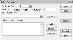
The Solver Parameters dialog box will appear, as shown in Figure 27-2.
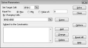
Click the Set Target Cell box and then select our profit cell (cell D12). Click the By Changing Cells box and then point to the range D2:I2, which contains the pounds produced of each drug. The dialog box should now look Figure 27-3.
We’re now ready to add constraints to the model. Click the Add button. You’ll see the Add Constraint dialog box, shown in Figure 27-4.


Adding these constraints ensures that when Solver tries different combinations for the changing cell values, only combinations that satisfy the following parameters will be considered:
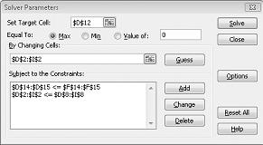
Click OK in the Add Constraint dialog box. The Solver window should look like Figure 27-7.
We enter the constraint that changing cells must be non-negative in the Solver Options dialog box. Click the Options button in the Solver Parameters dialog box. Check the Assume Linear Model box and the Assume Non-Negative box, as shown in Figure 27-8 on the next page. Click OK.
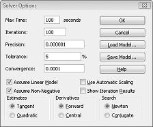
Checking the Assume Non-Negative box ensures that Solver considers only combinations of changing cells in which each changing cell assumes a non-negative value. We checked the Assume Linear Model box because the product mix problem is a special type of Solver problem called a linear model. Essentially, a Solver model is linear under the following conditions:
Why is this Solver problem linear? Our target cell (profit) is computed as
(Drug 1 profit per pound)*(Drug 1 pounds produced) +
(Drug 2 profit per pound)*(Drug 2 pounds produced) + .
(Drug 6 profit per pound)*(Drug 6 pounds produced)
This computation follows a pattern in which the target cell’s value is derived by adding together terms of the form (changing cell)*(constant).
Our labor constraint is evaluated by comparing the value derived from (Labor used per pound of Drug 1)*(Drug 1 pounds produced) + (Labor used per pound of Drug 2)*(Drug 2 pounds produced)+ …(Labor used per pound of Drug 6)*(Drug 6 pounds produced) to the labor available.
Therefore, the labor constraint is evaluated by adding together the terms of the form (changing cell)*(constant) and comparing the sums to a constant. Both the labor constraint and the raw material constraint satisfy the linear model requirement.
Our demand constraints take the form
Each demand constraint also satisfies the linear model requirement, because each is evaluated by adding together the terms of the form (changing cell)*(constant) and comparing the sums to a constant.
Having shown that our product mix model is a linear model, why should we care?
After clicking OK in the Solver Options dialog box, we return to the main Solver dialog box, shown earlier in Figure 27-7. When we click Solve, Solver calculates an optimal solution (if one exists) for our product mix model. As I stated in Chapter 26, an optimal solution to the product mix model would be a set of changing cell values (pounds produced of each drug) that maximizes profit over the set of all feasible solutions. Again, a feasible solution is a set of changing cell values satisfying all constraints. The changing cell values shown in Figure 27-9 are a feasible solution because all production levels are non-negative, production levels do not exceed demand, and resource usage does not exceed available resources.
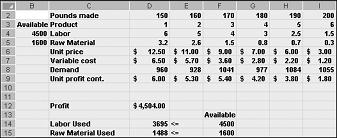
The changing cell values shown in Figure 27-10 on the next page represent an infeasible solution for the following reasons:
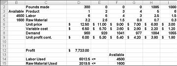
After clicking Solve, Solver quickly finds the optimal solution shown in Figure 27-11. You need to select Keep Solver Solution to preserve the optimal solution values in the worksheet.
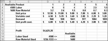
Our drug company can maximize its monthly profit at a level of $6,625.20 by producing 596.67 pounds of Drug 4, 1084 pounds of Drug 5, and none of the other drugs! We can’t determine if we can achieve the maximum profit of $6,625.20 in other ways. All we can be sure of is that with our limited resources and demand, there is no way to make more than $6,627.20 this month.
Does a Solver model always have a solution?Suppose that demand for each product must be met. (See the No Feasible Solution worksheet in the file Prodmix.xlsx.) We then have to change our demand constraints from D2:I2 to D2:I2>=D8:I8. To do this, open Solver, select the D2:I2

Select >=, and then click OK. We’ve now ensured that Solver will consider changing only cell values that meet all demands. When you click Solve, you’ll see the message "Solver could not find a feasible solution." This message does not mean that we made a mistake in our model, but rather that with our limited resources, we can’t meet demand for all products. Solver is simply telling us that if we want to meet demand for each product, we need to add more labor, more raw materials, or more of both.